Python Examples

To learn more about Python, check out my open-access textbook Minimalist Data Wrangling in Python.

How to Install

To install the package from PyPI, call:

pip3 install lumbermark  # python3 -m pip install lumbermark

Basic Use

Note

This section is a work in progress. In the meantime, take a look at the examples in the reference manual.

import numpy as np
import pandas as pd
import matplotlib.pyplot as plt
import deadwood

def plot_scatter(X, labels=None):
    deadwood.plot_scatter(X, asp=1, labels=labels, alpha=0.75, markers='o', s=10)

wut/z2 is an example dataset with five clusters of rather non-homogeneous densities. Lumbermark separates them correctly with no need for further parameter tuning:

import lumbermark
Z2 = np.loadtxt("z2.data.gz", ndmin=2)
lmark = lumbermark.Lumbermark(n_clusters=5)
labels = lmark.fit_predict(Z2)
plot_scatter(Z2, labels)
plt.show()

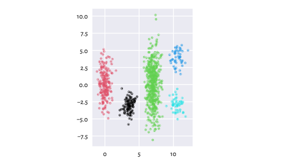
Figure 1 The clustered z2 dataset

Note the scikit-learn-compatible API.

Outlier Detection in the Case of Clusters of Heterogeneous Densities

The recently-developed Deadwood outlier detection algorithm works quite well in the case of clusters of similar densities. However, we can combine it with Lumbermark to detect outliers in each detected cluster separately.

plt.subplot(121)
is_outlier_homo   = deadwood.Deadwood().fit_predict(Z2)
plot_scatter(Z2, (is_outlier_homo<0))
plt.title("Deadwood")

plt.subplot(122)
is_outlier_hetero = deadwood.Deadwood().fit_predict(lmark)
plot_scatter(Z2, (is_outlier_hetero<0))
plt.title("Deadwood+Lumbermark")

plt.show()

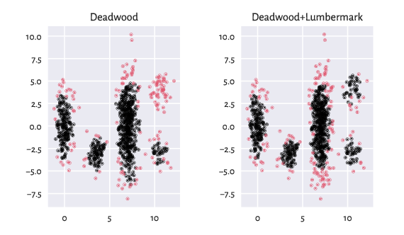
Figure 2 Outlier detection of the z2 dataset

Run Times

Thanks to quitefastmst, the time to perform a cluster analysis is pretty low in spaces of low intrinsic dimensionality.

Let’s conduct a test on a dataset consisting of 1M points in \(\mathbb{R}^2\):

import time
import numpy as np
np.random.seed(123)
n = 1_000_000
d = 2
X = np.random.randn(n, d)

Lumbermark:

import lumbermark
t0 = time.time()
l = lumbermark.Lumbermark(n_clusters=2)
l.fit(X)
print("Elapsed time: %.2f secs." % (time.time()-t0))
## Lumbermark()
## Elapsed time: 1.49 secs.

Due to the curse of dimensionality, processing datasets with high intrinsic dimensionality is slower.

A comparison against k-means (usually the fastest algorithm for small k):

import sklearn.cluster
t0 = time.time()
k = sklearn.cluster.KMeans(n_clusters=2)
k.fit(X)
print("Elapsed time: %.2f secs." % (time.time()-t0))
## KMeans(n_clusters=2)
## Elapsed time: 0.18 secs.

A comparison against Genie:

import genieclust
t0 = time.time()
g = genieclust.Genie(n_clusters=2)
g.fit(X)
print("Elapsed time: %.2f secs." % (time.time()-t0))
## Genie(quitefastmst_params={})
## Elapsed time: 2.60 secs.

A comparison against fast_hdbscan:

import fast_hdbscan
t0 = time.time()
h = fast_hdbscan.HDBSCAN()
h.fit(X)
print("Elapsed time: %.2f secs." % (time.time()-t0))
## HDBSCAN()
## Elapsed time: 16.55 secs.